11. From Physics to Vegetation Traits: Hybrid Inversion

library(ToolsRTM)

Every tutorial so far ran the forward model: traits in, spectrum out. Inversion goes the other way – given ONLY the sensor-band reflectance a satellite or field spectrometer would measure, retrieve a biophysical trait (chlorophyll content, Cab, throughout this page) without knowing the ground truth. This is the hybrid approach: instead of solving the radiative transfer equations analytically (rarely possible) or field- calibrating an empirical index-to-trait relationship (needs field data per site/crop), simulate a LUT with the physics you already have, and learn the reflectance-to-trait relationship from the simulation itself.

Parameter LUT
     |
     v
RTM simulations (Tutorials 01-06)
     |
     v
Sensor convolution (Tutorial 07)
     |
     v
Synthetic training dataset (reflectance, trait) pairs
     |
     v
Inversion method
     |
     v
Vegetation traits

Three inversion methods share this exact framework, differing only in the last step:

get.inversionOpt() (this page): no model is fit at all. It ranks every spectrum in a reference LUT by how closely it matches an observed spectrum under a chosen merit function, then averages the trait values of the closest matches. Pure library search.
get.inversion() (Tutorial 12): fits a statistical/ML model (Random Forest, PLSR, SVM, … 12 algorithms via caret) on a training LUT, then predicts on new spectra.
getMLmodel() (Tutorial 13): fits a deep-learning model on the same kind of data.

1. Simulate a LUT and convolve to Sentinel-2A

n_samples <- 700
LUT <- as.data.frame(getLUT(inputs = ToolsRTM::inputsPROSAIL, nLUT = n_samples, setseed = 1))

wl <- 400:2500
rsoil <- rep(0.15, length(wl))
refl <- t(sapply(seq_len(n_samples), function(i) {
  foursail(inputLUT = LUT[i, ], rsoil = rsoil, LeafModel = "PROSPECT-PRO")$rsot
}))

refl_X <- as.data.frame(refl); colnames(refl_X) <- paste0("X", wl); refl_X <- cbind(id = seq_len(nrow(refl_X)), refl_X)
se2a <- suppressMessages(get.spectra.convolved(rfl = refl_X, sensor = "Sentinel2a", plot.spectra = FALSE))
#> [1] "Spectral resampling function to SENTINEL2A is being processed ..."
#>   |                                                                              |                                                                      |   0%  |                                                                              |=====                                                                 |   8%  |                                                                              |===========                                                           |  15%  |                                                                              |================                                                      |  23%  |                                                                              |======================                                                |  31%  |                                                                              |===========================                                           |  38%  |                                                                              |================================                                      |  46%  |                                                                              |======================================                                |  54%  |                                                                              |===========================================                           |  62%  |                                                                              |================================================                      |  69%  |                                                                              |======================================================                |  77%  |                                                                              |===========================================================           |  85%  |                                                                              |=================================================================     |  92%  |                                                                              |======================================================================| 100%
wl_bands <- as.numeric(names(se2a)[-1])
band_names <- paste0("B", seq_along(wl_bands))
names(se2a) <- c("id", band_names)

700 simulated spectra, convolved to Sentinel-2A’s 13 real bands – this is what every inversion method below actually sees, not the native 1nm spectrum.

2. A train/test split, shared by every method

set.seed(1)
train_idx <- sample(seq_len(n_samples), size = round(0.7 * n_samples))
test_idx  <- setdiff(seq_len(n_samples), train_idx)

LUT_train <- LUT[train_idx, ]; LUT_test <- LUT[test_idx, ]
se2a_mat <- as.matrix(se2a[, band_names])
se2a_train_mat <- se2a_mat[train_idx, ]; se2a_test_mat <- se2a_mat[test_idx, ]

r2_f   <- function(obs, pred) 1 - sum((obs - pred)^2) / sum((obs - mean(obs))^2)
rmse_f <- function(obs, pred) sqrt(mean((obs - pred)^2))

cat("Train:", length(train_idx), "spectra. Test (held out):", length(test_idx), "spectra.\n")
#> Train: 490 spectra. Test (held out): 210 spectra.

3. `get.inversionOpt()`: LUT merit-function matching

method picks how “closeness” between two spectra is measured. nOpt controls how many of the closest training spectra get averaged together for the final trait estimate:

opt_rmse <- get.inversionOpt(rfl.sensor = se2a_test_mat, rfl.rtm = se2a_train_mat,
                              LUT = LUT_train, wave = wl_bands, method = "merit-RMSE", nOpt = 5)
opt_fge  <- get.inversionOpt(rfl.sensor = se2a_test_mat, rfl.rtm = se2a_train_mat,
                              LUT = LUT_train, wave = wl_bands, method = "merit-FGE", nOpt = 5)
opt_dwt  <- get.inversionOpt(rfl.sensor = se2a_test_mat, rfl.rtm = se2a_train_mat,
                              LUT = LUT_train, wave = wl_bands, method = "merit-DWT", nOpt = 5)

Each call returns a 2-element list: [[1]] (rfl.b) is the matched reflectance itself, [[2]] (LUT.best) is the corresponding trait table:

opt_metrics <- data.frame(
  method = c("merit-RMSE", "merit-FGE", "merit-DWT"),
  R2   = c(r2_f(LUT_test$Cab, opt_rmse[[2]]$Cab), r2_f(LUT_test$Cab, opt_fge[[2]]$Cab), r2_f(LUT_test$Cab, opt_dwt[[2]]$Cab)),
  RMSE = c(rmse_f(LUT_test$Cab, opt_rmse[[2]]$Cab), rmse_f(LUT_test$Cab, opt_fge[[2]]$Cab), rmse_f(LUT_test$Cab, opt_dwt[[2]]$Cab))
)
knitr::kable(opt_metrics, digits = 3)

method	R2	RMSE
merit-RMSE	0.573	10.895
merit-FGE	0.648	9.902
merit-DWT	0.533	11.401

merit-RMSE/merit-FGE compare raw band reflectance; merit-DWT compares each spectrum’s discrete wavelet transform coefficients instead (sensitive to overall spectral shape rather than each band’s exact value). merit-NRMSE, merit-MAE, merit-NMB, and merit-1stD (first-derivative matching) are the remaining built-in options; custom_stat accepts your own function(sim, obs).

plot(LUT_test$Cab, opt_rmse[[2]]$Cab, pch = 19, col = "#2166AC",
     xlab = "Observed Cab", ylab = "Predicted Cab (merit-RMSE, nOpt=5)",
     main = "LUT merit-function matching")
abline(0, 1, col = "grey40", lty = 2)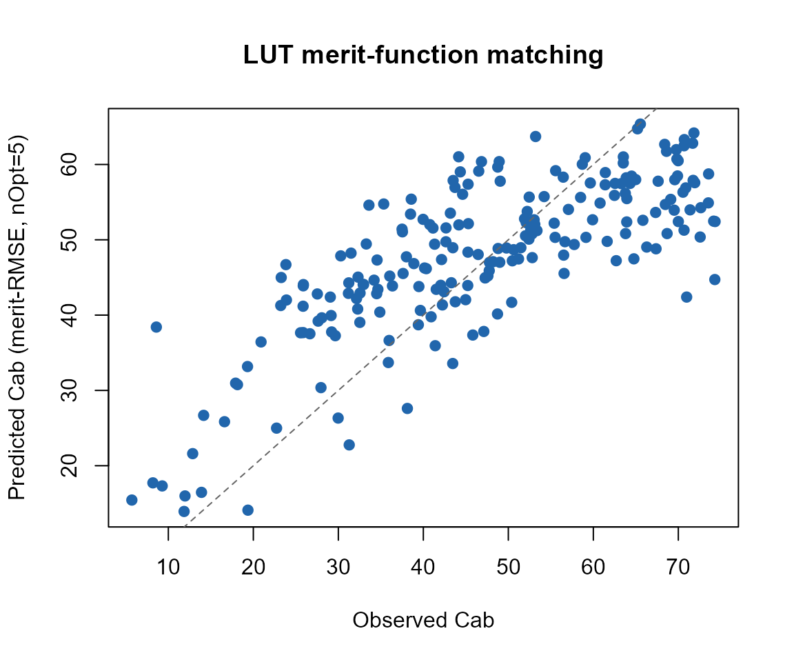

Why this method, and when

get.inversionOpt() needs no training step – a quick, physically- grounded retrieval with no ML infrastructure. Its limitation: accuracy is capped by how well the reference LUT covers the true trait space, and it re-searches the whole reference LUT for every new observation (no learned model to reuse). Tutorial 12 builds actual fitted models instead, trading that simplicity for better accuracy at scale.

4. Is 700 samples actually enough?

A LUT-search method’s accuracy is capped by how densely its reference LUT covers the trait space; PROSAIL-hybrid-inversion literature typically recommends LUT sizes in the thousands (often tens of thousands for operational retrieval) for reliable coverage of even a handful of free parameters. 700 rows – 490 of them used as the search reference after the train/test split – is a real step up from a bare-minimum demo size, but still short of that. To make the effect concrete rather than just cite a number, here is get.inversionOpt() run at 100 rows, at this page’s own 700, and at a 2000-row reference:

run_experiment <- function(n_samples, seed = 1) {
  LUT_n <- as.data.frame(getLUT(inputs = ToolsRTM::inputsPROSAIL, nLUT = n_samples, setseed = seed))
  refl_n <- t(sapply(seq_len(n_samples), function(i) {
    foursail(inputLUT = LUT_n[i, ], rsoil = rsoil, LeafModel = "PROSPECT-PRO")$rsot
  }))
  refl_X_n <- as.data.frame(refl_n); colnames(refl_X_n) <- paste0("X", wl)
  refl_X_n <- cbind(id = seq_len(nrow(refl_X_n)), refl_X_n)
  se2a_n <- suppressMessages(get.spectra.convolved(rfl = refl_X_n, sensor = "Sentinel2a", plot.spectra = FALSE))
  names(se2a_n) <- c("id", band_names)

  set.seed(seed)
  train_idx_n <- sample(seq_len(n_samples), size = round(0.7 * n_samples))
  test_idx_n  <- setdiff(seq_len(n_samples), train_idx_n)
  se2a_n_mat <- as.matrix(se2a_n[, band_names])

  opt_n <- get.inversionOpt(rfl.sensor = se2a_n_mat[test_idx_n, ], rfl.rtm = se2a_n_mat[train_idx_n, ],
                             LUT = LUT_n[train_idx_n, ], wave = wl_bands, method = "merit-RMSE", nOpt = 5)
  data.frame(n = n_samples, n_train = length(train_idx_n),
             R2 = r2_f(LUT_n[test_idx_n, ]$Cab, opt_n[[2]]$Cab),
             RMSE = rmse_f(LUT_n[test_idx_n, ]$Cab, opt_n[[2]]$Cab))
}
sample_size_results <- rbind(run_experiment(100), run_experiment(700), run_experiment(2000))

knitr::kable(sample_size_results, digits = 3, row.names = FALSE)

n	n_train	R2	RMSE
100	70	-0.080	15.183
700	490	0.573	10.895
2000	1400	0.648	9.465

At 100 samples, R² is negative – the method has no real skill, worse than just guessing the mean. Jumping to 700 – this page’s own LUT size – turns that into real, usable skill (R² = 0.573): the biggest single gain sits in that first jump, not in going further. Continuing to 2000 still helps (R² = 0.648, lower RMSE) but by a much smaller margin than 100-to-700 did – diminishing returns have clearly set in by 700 rows, even though 700 remains short of the “thousands” literature recommendation. 700 rows is a reasonable balance for a tutorial that still needs to build in a reasonable time: enough to demonstrate a real, usable hybrid-inversion result, not just the theory. For actual applications, especially with more than one free parameter to retrieve simultaneously, still build a LUT of at least a few thousand rows (Tutorial 06 covers parallelizing exactly that).

What’s next