12. Comparing ML Algorithms for RTM Inversion
t12-ml-inversion-comparison.Rmd
library(ToolsRTM)Tutorial 11 covered get.inversionOpt() – pure
LUT-search, no model fit at all. This page introduces
get.inversion() for the first time, and compares several of
its 12 supported algorithms (via caret) on the same
LUT/train-test split, so the comparison is apples-to-apples.
1. Same LUT, same split as Tutorial 11
n_samples <- 700
LUT <- as.data.frame(getLUT(inputs = ToolsRTM::inputsPROSAIL, nLUT = n_samples, setseed = 1))
wl <- 400:2500
rsoil <- rep(0.15, length(wl))
refl <- t(sapply(seq_len(n_samples), function(i) {
  foursail(inputLUT = LUT[i, ], rsoil = rsoil, LeafModel = "PROSPECT-PRO")$rsot
}))
refl_X <- as.data.frame(refl); colnames(refl_X) <- paste0("X", wl); refl_X <- cbind(id = seq_len(nrow(refl_X)), refl_X)
se2a <- suppressMessages(get.spectra.convolved(rfl = refl_X, sensor = "Sentinel2a", plot.spectra = FALSE))
#> [1] "Spectral resampling function to SENTINEL2A is being processed ..."
#>   |                                                                              |                                                                      |   0%  |                                                                              |=====                                                                 |   8%  |                                                                              |===========                                                           |  15%  |                                                                              |================                                                      |  23%  |                                                                              |======================                                                |  31%  |                                                                              |===========================                                           |  38%  |                                                                              |================================                                      |  46%  |                                                                              |======================================                                |  54%  |                                                                              |===========================================                           |  62%  |                                                                              |================================================                      |  69%  |                                                                              |======================================================                |  77%  |                                                                              |===========================================================           |  85%  |                                                                              |=================================================================     |  92%  |                                                                              |======================================================================| 100%
band_names <- paste0("B", seq_along(as.numeric(names(se2a)[-1])))
names(se2a) <- c("id", band_names)

set.seed(1)
train_idx <- sample(seq_len(n_samples), size = round(0.7 * n_samples))
test_idx  <- setdiff(seq_len(n_samples), train_idx)
train_df <- cbind(LUT[train_idx, ], se2a[train_idx, band_names])
test_df  <- cbind(LUT[test_idx, ],  se2a[test_idx,  band_names])

r2_f   <- function(obs, pred) 1 - sum((obs - pred)^2) / sum((obs - mean(obs))^2)
rmse_f <- function(obs, pred) sqrt(mean((obs - pred)^2))
matplot(wl, t(refl[sample(seq_len(n_samples), 30), ]), type = "l", lty = 1,
        col = adjustcolor("#0072B2", alpha.f = 0.3),
        xlab = "Wavelength (nm)", ylab = "TOC reflectance (rsot)",
        main = "30 of the 700 simulated spectra behind this LUT")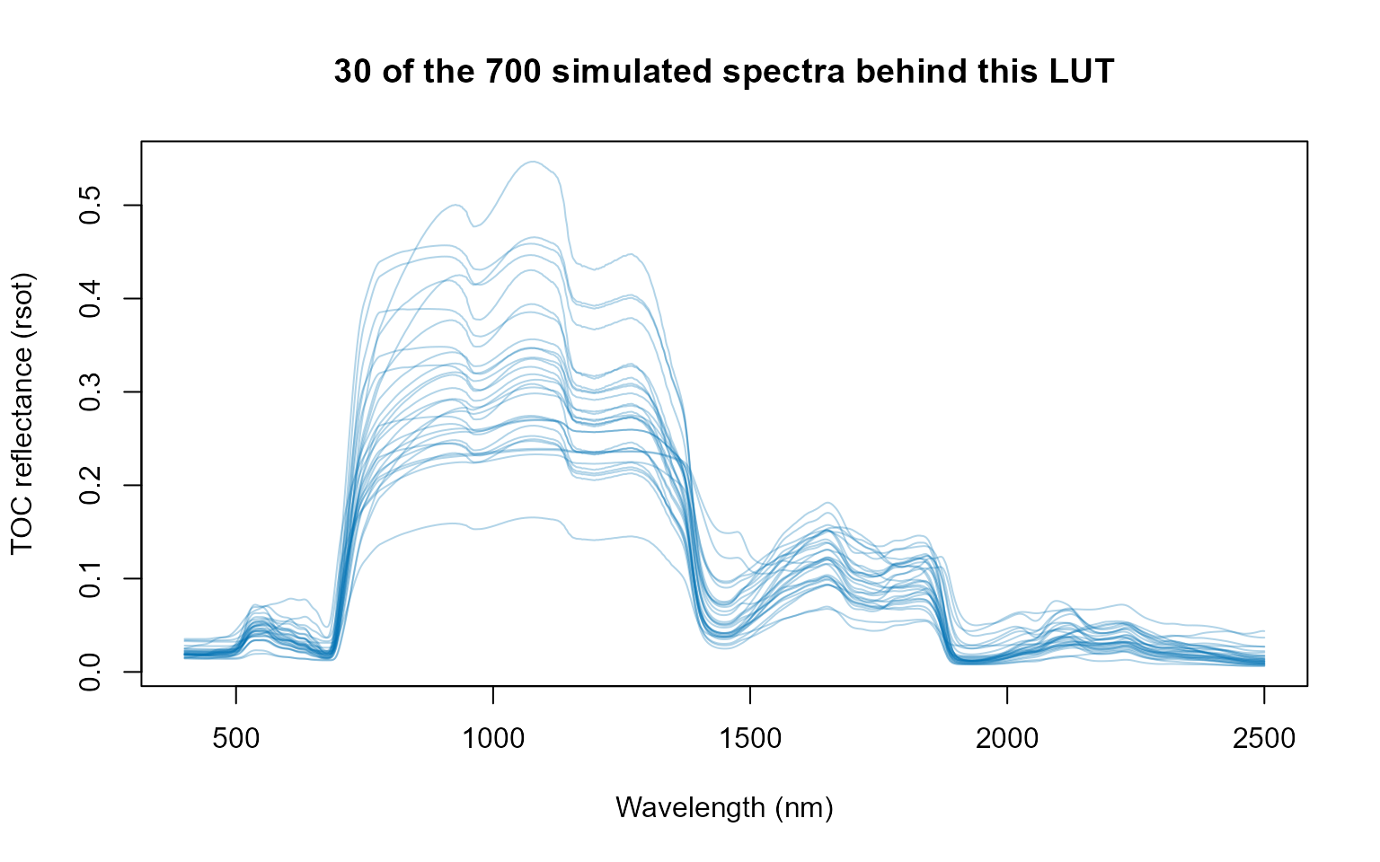
2. Fit several algorithms, predict Cab on the held-out test set
get.inversion() supports 12 algorithms:
"PLSR", "SVM", "RF",
"GB", "NN", "Bayesian",
"AdaBag", "BRNN", "xGB",
"RVM", "qLASSO", "Ensemble".
"NN" (caret’s nnet tuning grid) is skipped
here – impractically slow against this many predictors at caret’s
default tuning grid, the same reason this package’s own course pipeline
scripts (Scripts/R/*/2-inversion_ML.R) skip it too. A
representative subset run for real below; the rest of the call is
identical for any of the others.
"Ensemble" (stacks SVM + Gradient Boosting + a
neural net via caretEnsemble) is left out of the comparison
below on purpose: while verifying this page, it surfaced two
real bugs in get.inversion()‘s source (both fixed directly
in the package for this release – fmla.n was referenced
without being defined in that branch, and its internal
stackControl passed the whole training data.frame to
caret::createFolds() instead of the response column,
misaligning fold sizes) – but even after both fixes,
caretEnsemble::caretStack() still fails with
"pred_rows == pred_rows[1L] are not all TRUE", a deeper
row-alignment mismatch across the three stacked sub-models’ predictions
that needs further investigation into how their tuning grids interact,
not something safe to guess-fix here.
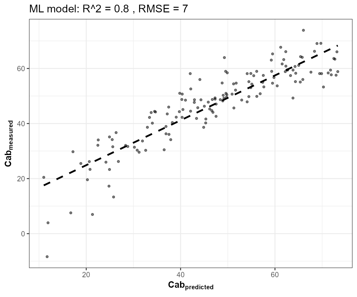
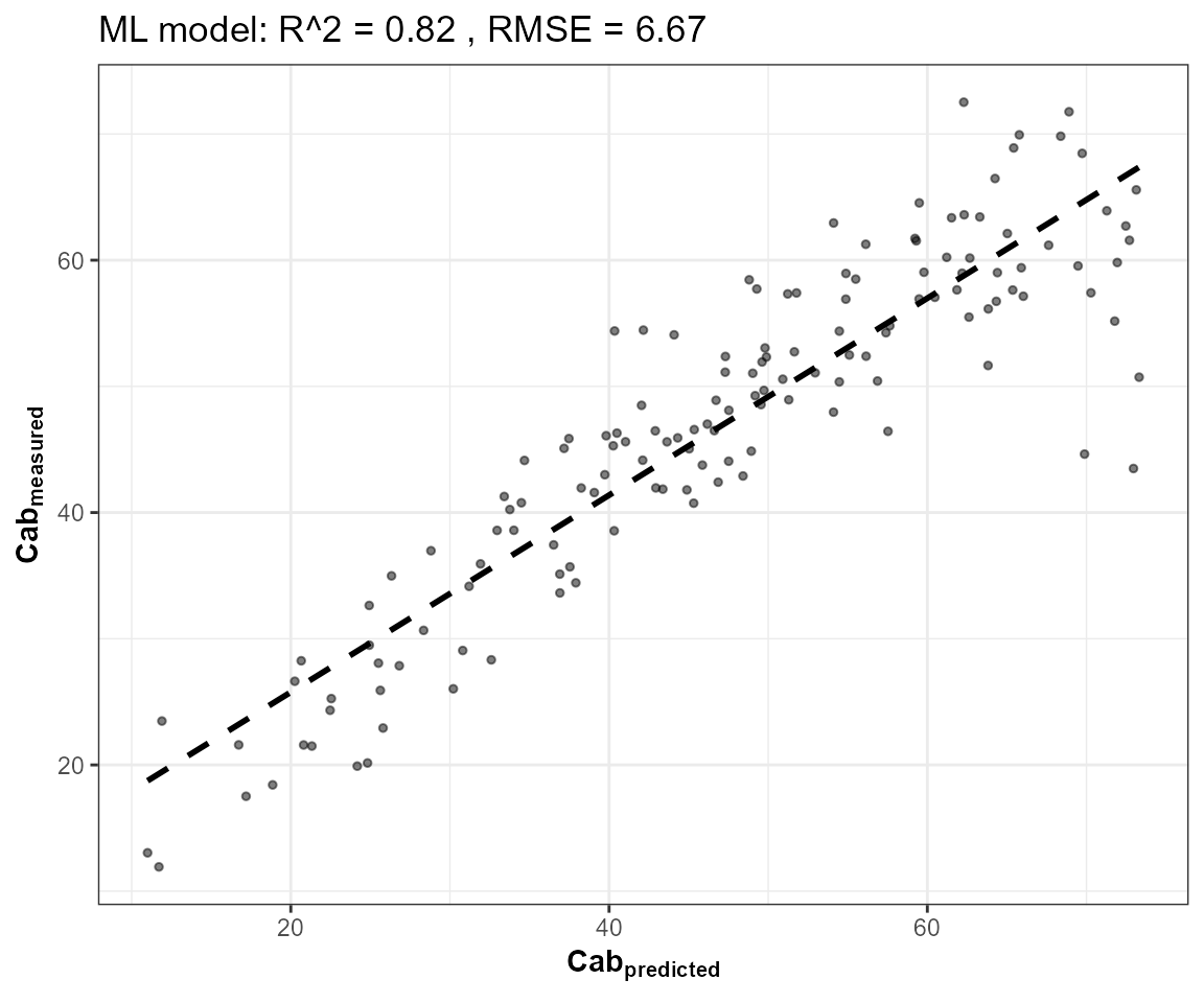
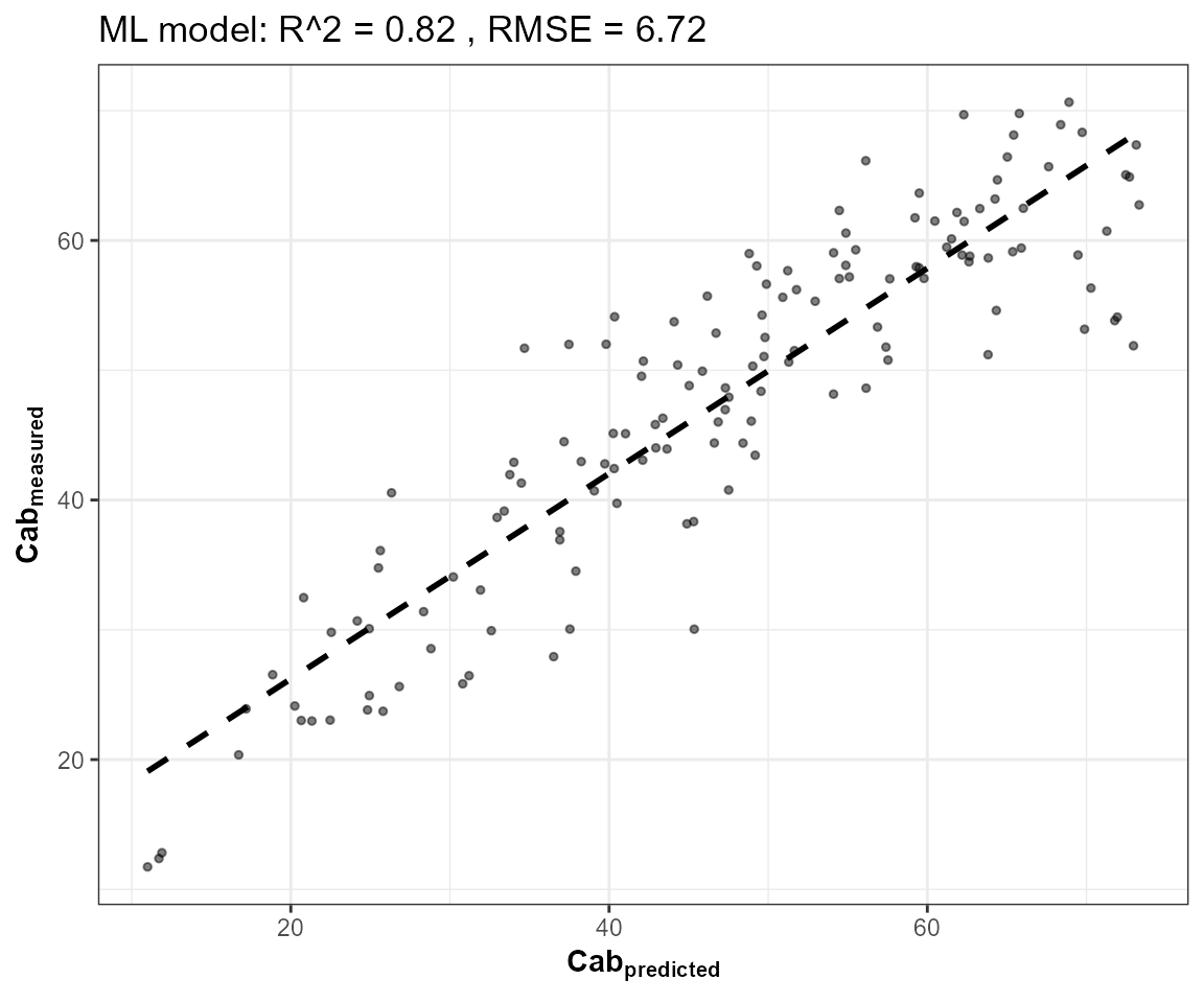
algorithms <- c("PLSR", "SVM", "RF", "GB")
fits <- lapply(algorithms, function(algo) {
  get.inversion(data = train_df, depVar = "Cab", inputs = band_names,
                algorithm = algo, n.samples = nrow(train_df), seed = 42)
})
names(fits) <- algorithms
metrics <- do.call(rbind, lapply(algorithms, function(algo) {
  pred <- as.numeric(predict(fits[[algo]]$model, newdata = test_df[, c("Cab", band_names)]))
  data.frame(algorithm = algo, R2 = r2_f(test_df$Cab, pred), RMSE = rmse_f(test_df$Cab, pred))
}))
knitr::kable(metrics[order(-metrics$R2), ], digits = 3, row.names = FALSE)| algorithm | R2 | RMSE |
|---|---|---|
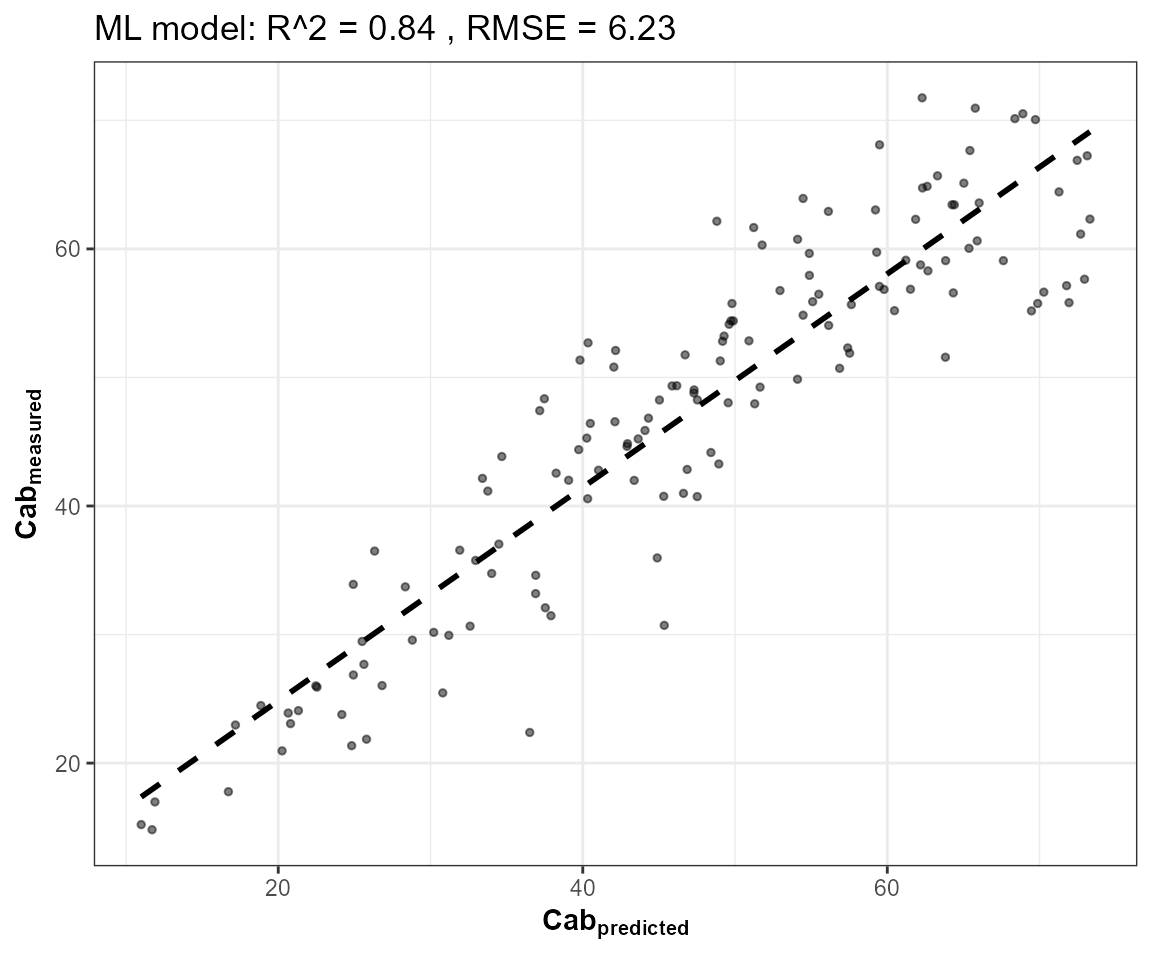
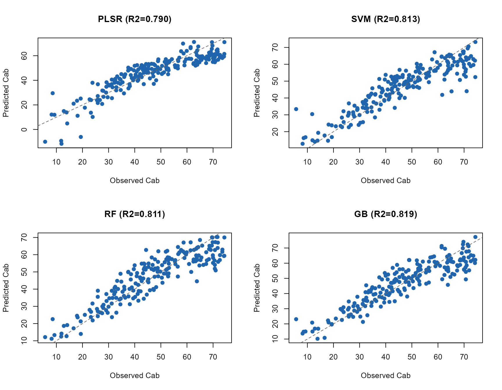
| GB | 0.819 | 7.096 |
| SVM | 0.813 | 7.223 |
| RF | 0.811 | 7.256 |
| PLSR | 0.790 | 7.648 |
best_algo <- metrics$algorithm[which.max(metrics$R2)]
pred_best <- as.numeric(predict(fits[[best_algo]]$model, newdata = test_df[, c("Cab", band_names)]))
plot(test_df$Cab, pred_best, pch = 19, col = "#2166AC",
     xlab = "Observed Cab", ylab = paste("Predicted Cab (", best_algo, ")"),
     main = paste("Best algorithm on this LUT:", best_algo))
abline(0, 1, col = "grey40", lty = 2)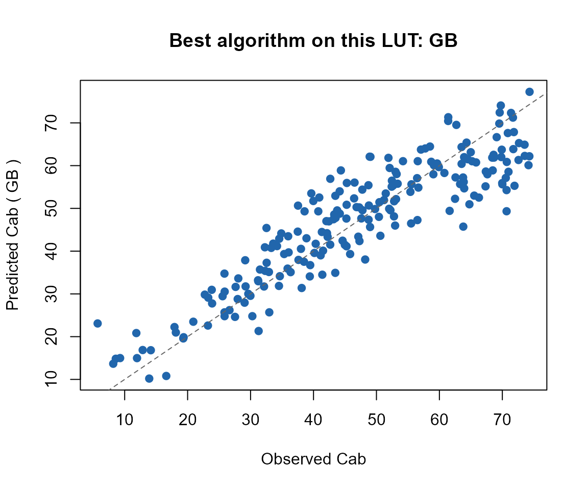
All four algorithms, not just the winner
A single “best” scatter plot hides how the others actually did. Every algorithm’s predicted-vs-observed, side by side, plus the R2/RMSE bars from Section 2’s table:
op <- par(mfrow = c(2, 2))
for (algo in algorithms) {
  pred <- as.numeric(predict(fits[[algo]]$model, newdata = test_df[, c("Cab", band_names)]))
  r2_here <- round(r2_f(test_df$Cab, pred), 3)
  plot(test_df$Cab, pred, pch = 19, col = "#2166AC",
       xlab = "Observed Cab", ylab = "Predicted Cab",
       main = sprintf("%s (R2=%.3f)", algo, r2_here))
  abline(0, 1, col = "grey40", lty = 2)
}
par(op)
op <- par(mfrow = c(1, 2))
barplot(setNames(metrics$R2, metrics$algorithm), col = "#0072B2", ylab = "R2", main = "R2 by algorithm")
barplot(setNames(metrics$RMSE, metrics$algorithm), col = "#D55E00", ylab = "RMSE", main = "RMSE by algorithm")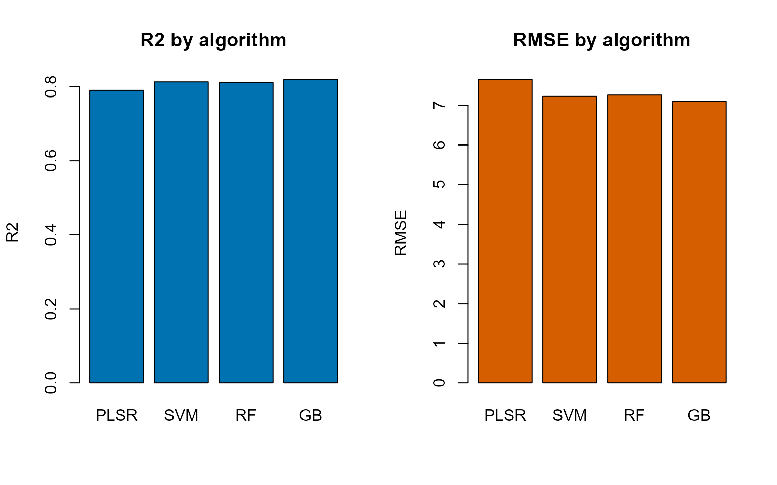
par(op)3. Comparing against Tutorial 11’s merit-function matching
se2a_mat <- as.matrix(se2a[, band_names])
opt_rmse <- get.inversionOpt(rfl.sensor = se2a_mat[test_idx, ], rfl.rtm = se2a_mat[train_idx, ],
                              LUT = LUT[train_idx, ], wave = as.numeric(sub("B", "", band_names)),
                              method = "merit-RMSE", nOpt = 5)
comparison <- rbind(metrics[, c("algorithm", "R2", "RMSE")],
                     data.frame(algorithm = "inversionOpt (merit-RMSE)",
                                R2 = r2_f(LUT[test_idx, ]$Cab, opt_rmse[[2]]$Cab),
                                RMSE = rmse_f(LUT[test_idx, ]$Cab, opt_rmse[[2]]$Cab)))
knitr::kable(comparison[order(-comparison$R2), ], digits = 3, row.names = FALSE)| algorithm | R2 | RMSE |
|---|---|---|
| GB | 0.819 | 7.096 |
| SVM | 0.813 | 7.223 |
| RF | 0.811 | 7.256 |
| PLSR | 0.790 | 7.648 |
| inversionOpt (merit-RMSE) | 0.573 | 10.895 |
At this LUT size (700 rows, 490 training), the fitted ML models
already have a clear edge over pure LUT-search – every algorithm here
beats get.inversionOpt()’s R2 of 0.573 by a real margin
(0.79-0.82). A fitted model extracts more from the same reference set
than nearest-match search alone; that gap tends to widen further with
more training data, and narrows (or reverses) in
get.inversionOpt()’s favour only when too little data is
available to fit a model reliably (Tutorial 11’s discussion of when to
use which).
4. Multiple traits: do spectral indices actually help?
Every comparison so far predicted one trait (Cab) from raw bands alone. Real applications need several traits, and raw reflectance bands are not the only useful input – vegetation indices (Tutorial 09) can carry trait-specific signal that a generic ML algorithm has to work harder to reconstruct from bands on its own. This section checks that directly, on the same LUT and train/test split, across six traits: Random Forest fit twice per trait – bands only, and bands plus a small, per-trait selection of the indices most correlated with that specific trait (not one fixed index set reused everywhere).
# Real Sentinel-2A band names (not the generic B1..B10 from Section 1) --
# getIndicesSE2.ML()'s index formulas need to find specific bands like
# B8A/B11/B12 by name.
se2a_full <- suppressMessages(get.spectra.convolved(rfl = refl_X, sensor = "Sentinel2a", plot.spectra = FALSE))
#> [1] "Spectral resampling function to SENTINEL2A is being processed ..."
#> | | | 0% | |===== | 8% | |=========== | 15% | |================ | 23% | |====================== | 31% | |=========================== | 38% | |================================ | 46% | |====================================== | 54% | |=========================================== | 62% | |================================================ | 69% | |====================================================== | 77% | |=========================================================== | 85% | |================================================================= | 92% | |======================================================================| 100%
names(se2a_full) <- c("id", "B1","B2","B3","B4","B5","B6","B7","B8","B8A","B9","B10","B11","B12")
bands_real <- c("B2","B3","B4","B5","B6","B7","B8","B8A","B11","B12") # skip the atmospheric-only bands (B1, B9, B10)
idx_ml <- suppressMessages(getIndicesSE2.ML(df = se2a_full[, -1], sensor = "Sentinel-2a", df.data = NULL, fast.process = TRUE))
#> | | | 0% | | | 1% | |= | 1% | |= | 2% | |== | 2% | |== | 3% | |=== | 4% | |=== | 5% | |==== | 5% | |==== | 6% | |===== | 6% | |===== | 7% | |===== | 8% | |====== | 8% | |====== | 9% | |======= | 9% | |======= | 10% | |======= | 11% | |======== | 11% | |======== | 12% | |========= | 12% | |========= | 13% | |========== | 14% | |========== | 15% | |=========== | 15% | |=========== | 16% | |============ | 16% | |============ | 17% | |============ | 18% | |============= | 18% | |============= | 19% | |============== | 19% | |============== | 20% | |============== | 21% | |=============== | 21% | |=============== | 22% | |================ | 22% | |================ | 23% | |================= | 24% | |================= | 25% | |================== | 25% | |================== | 26% | |=================== | 26% | |=================== | 27% | |=================== | 28% | |==================== | 28% | |==================== | 29% | |===================== | 29% | |===================== | 30% | |===================== | 31% | |====================== | 31% | |====================== | 32% | |======================= | 32% | |======================= | 33% | |======================== | 34% | |======================== | 35% | |========================= | 35% | |========================= | 36% | |========================== | 36% | |========================== | 37% | |========================== | 38% | |=========================== | 38% | |=========================== | 39% | |============================ | 39% | |============================ | 40% | |============================ | 41% | |============================= | 41% | |============================= | 42% | |============================== | 42% | |============================== | 43% | |=============================== | 44% | |=============================== | 45% | |================================ | 45% | |================================ | 46% | |================================= | 46% | |================================= | 47% | |================================= | 48% | |================================== | 48% | |================================== | 49% | |=================================== | 49% | |=================================== | 50% | |=================================== | 51% | |==================================== | 51% | |==================================== | 52% | |===================================== | 52% | |===================================== | 53% | |===================================== | 54% | |====================================== | 54% | |====================================== | 55% | |======================================= | 55% | |======================================= | 56% | |======================================== | 57% | |======================================== | 58% | |========================================= | 58% | |========================================= | 59% | |========================================== | 59% | |========================================== | 60% | |========================================== | 61% | |=========================================== | 61% | |=========================================== | 62% | |============================================ | 62% | |============================================ | 63% | |============================================ | 64% | |============================================= | 64% | |============================================= | 65% | |============================================== | 65% | |============================================== | 66% | |=============================================== | 67% | |=============================================== | 68% | |================================================ | 68% | |================================================ | 69% | |================================================= | 69% | |================================================= | 70% | |================================================= | 71% | |================================================== | 71% | |================================================== | 72% | |=================================================== | 72% | |=================================================== | 73% | |=================================================== | 74% | |==================================================== | 74% | |==================================================== | 75% | |===================================================== | 75% | |===================================================== | 76% | |====================================================== | 77% | |====================================================== | 78% | |======================================================= | 78% | |======================================================= | 79% | |======================================================== | 79% | |======================================================== | 80% | |======================================================== | 81% | |========================================================= | 81% | |========================================================= | 82% | |========================================================== | 82% | |========================================================== | 83% | |========================================================== | 84% | |=========================================================== | 84% | |=========================================================== | 85% | |============================================================ | 85% | |============================================================ | 86% | |============================================================= | 87% | |============================================================= | 88% | |============================================================== | 88% | |============================================================== | 89% | |=============================================================== | 89% | |=============================================================== | 90% | |=============================================================== | 91% | |================================================================ | 91% | |================================================================ | 92% | |================================================================= | 92% | |================================================================= | 93% | |================================================================= | 94% | |================================================================== | 94% | |================================================================== | 95% | |=================================================================== | 95% | |=================================================================== | 96% | |==================================================================== | 97% | |==================================================================== | 98% | |===================================================================== | 98% | |===================================================================== | 99% | |======================================================================| 99% | |======================================================================| 100%
cat("Candidate indices:", ncol(idx_ml), "\n")
#> Candidate indices: 30
traits <- c("Cab", "Car", "Anth", "LAI", "EWT", "Cbrown")
n_top <- 5  # indices kept per trait

# Correlation against training rows only, per trait -- an index useful for
# EWT is not necessarily useful for Anth, so this is computed separately
# for each trait rather than picking one index set for all of them.
select_indices <- function(trait) {
  cors <- sapply(names(idx_ml), function(nm) suppressWarnings(cor(idx_ml[train_idx, nm], LUT[train_idx, trait])))
  cors <- cors[is.finite(cors)]
  names(sort(abs(cors), decreasing = TRUE))[seq_len(min(n_top, length(cors)))]
}
selected <- setNames(lapply(traits, select_indices), traits)
knitr::kable(data.frame(trait = traits, top_indices = sapply(selected, paste, collapse = ", ")), row.names = FALSE)| trait | top_indices |
|---|---|
| Cab | NDRE, CR.red.nir.1, CIre, CR.red.nir, Datt1 |
| Car | NDRE, CR.red.nir.1, CIre, CR.red.nir, Datt1 |
| Anth | BF.Anth, GM1, TCARI, CR.Brown, TCARI_OSAVI |
| LAI | PSSRa, RedEg1, WDRVI, NDVI, CIgreen |
| EWT | NDWI, MNDVI, CR.SWIR, WET, NDWI2 |
| Cbrown | CR.red.nir.6, CR.red.nir, IRECI, BF.Anth, CR.red.nir.1 |
run_pair <- function(trait) {
  idx_cols <- selected[[trait]]
  df_bands <- cbind(LUT[trait], se2a_full[bands_real])
  df_full  <- cbind(df_bands, idx_ml[idx_cols])

  fit_bands <- get.inversion(data = df_bands[train_idx, ], depVar = trait, inputs = bands_real,
                              algorithm = "RF", n.samples = length(train_idx), seed = 42)
  fit_full  <- get.inversion(data = df_full[train_idx, ], depVar = trait, inputs = c(bands_real, idx_cols),
                              algorithm = "RF", n.samples = length(train_idx), seed = 42)

  pred_bands <- as.numeric(predict(fit_bands$model, newdata = df_bands[test_idx, c(trait, bands_real)]))
  pred_full  <- as.numeric(predict(fit_full$model,  newdata = df_full[test_idx,  c(trait, bands_real, idx_cols)]))

  data.frame(trait = trait,
             R2_bands_only = r2_f(LUT[test_idx, trait], pred_bands),
             R2_bands_plus_indices = r2_f(LUT[test_idx, trait], pred_full))
}
trait_results <- do.call(rbind, lapply(traits, run_pair))
trait_results$delta <- trait_results$R2_bands_plus_indices - trait_results$R2_bands_only| trait | R2_bands_only | R2_bands_plus_indices | delta |
|---|---|---|---|
| EWT | 0.593 | 0.921 | 0.328 |
| Cbrown | 0.603 | 0.854 | 0.251 |
| LAI | 0.613 | 0.651 | 0.039 |
| Cab | 0.786 | 0.819 | 0.032 |
| Car | 0.748 | 0.777 | 0.029 |
| Anth | 0.527 | 0.447 | -0.081 |
ord <- order(trait_results$delta)
barplot(rbind(trait_results$R2_bands_only[ord], trait_results$R2_bands_plus_indices[ord]),
        beside = TRUE, names.arg = trait_results$trait[ord],
        col = c("#999999", "#0072B2"), ylab = "R2 (independent test set)",
        main = "Bands only vs. bands + top-5 correlated indices, per trait")
legend("topleft", c("Bands only", "+ indices"), fill = c("#999999", "#0072B2"), bty = "n")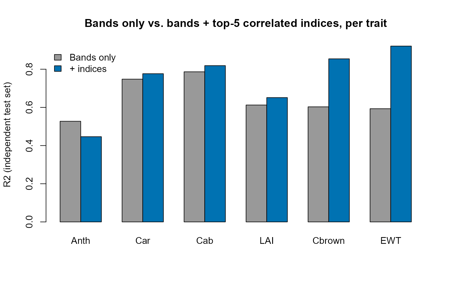
Adding indices helps most traits here, but not universally,
and by very different amounts. EWT and
Cbrown gain the most – unsurprising, since water- and
senescence-sensitive indices (built from SWIR bands the raw per-band RF
split has to rediscover on its own) target exactly that signal directly.
Cab/Car/LAI gain a real but more
modest amount – RF was already extracting a fair fraction of the
available structure from the bands alone. Anth is the one
exception: adding its top-5 correlated indices actually hurts
accuracy here (R2 0.527 -> 0.447). Anth is already the
weakest bands-only predictor of the six, consistent with anthocyanin’s
famously subtle spectral footprint (Tutorial 09); the indices most
correlated with it on the training split look like they’re picking up
incidental correlation rather than real signal, handing RF extra noisy
predictors instead of useful ones. The lesson generalises past this
specific LUT, and cuts sharper than before: which indices to
add, computed and selected per trait, matters more than adding indices
in general – and for a trait with a weak physical signal to begin with,
“most correlated on the training set” is not automatically the same as
“actually useful.”
What’s next
-
Tutorial 13 – deep learning
(
getMLmodel()) on the same kind of data, and when it’s worth the extra complexity over the algorithms here. - Tutorial 14 – this whole simulate-convolve-invert chain as one coherent pipeline, across every canopy model this package supports.